
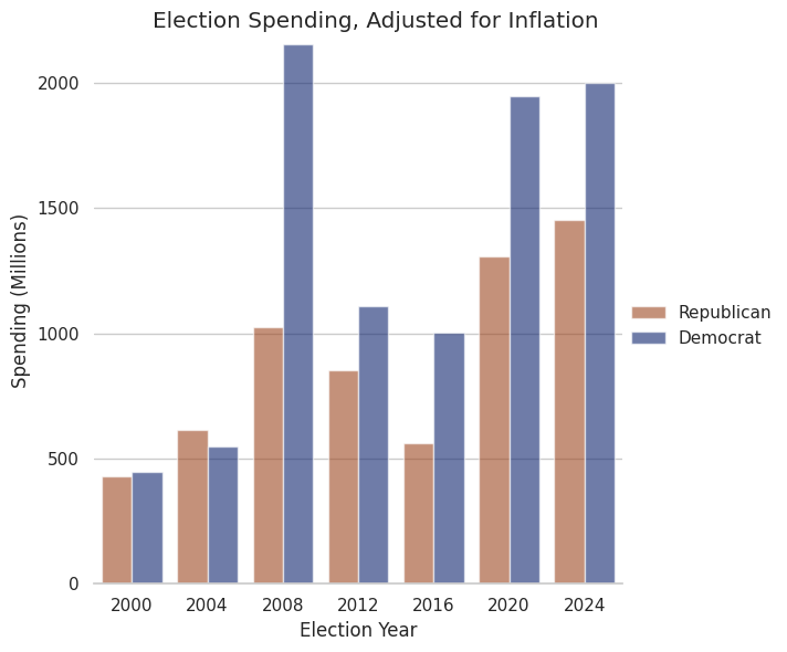
I’ll be the first to admit, I’ve massaged the data. There are simply not enough data points to produce good averages, and I’ve made assumptions, such as the normality of data. I started at the 2000 election, however really 2008 is when modern campaign finance began. We also have to work around the fact the data isn’t independent, or that campaign spending laws may change in ways I can’t account for (such as the McCain–Feingold Act of 2002).
That said, we have seen election spending seemingly have very little impact on elections. The last three elections were won by the candidate with the least money, with the winner being outspent by hundreds of millions.
But first: what is a p-value?
As you may not recall from your high school stats class, a p-value is the likelihood of observing data which is at least as extreme as what was observed. When our p-value is low, we call it statistically significant. Our data is being compared against the null hypothesis (H_0), which is assumed true, and the alternative hypothesis (H_1). A p-value < 0.05 means our data is statistically significant, meaning our results "extreme" if H_0 is true; a p-value < 0.01 is highly statistically significant.
Conversely, a p-value > 0.95 suggests statistical significance in favor of the null hypothesis, and p-value > 0.99 is highly statistically significant. When looking at election data and comparing it against funding, I came up with these hypotheses:
- H_0: There is no relationship between campaign funding and winning
- H_1: There is a relationship between campaign funding and winning
I will use these for all of the statistical tests.
Point-Biserial Correlation
A point-biserial correlation test is a good way to compare a continuous variable (in the case campaign spending) with a binary, or dichotomous, variable (which will be winning or losing the election). The continuous variable additionally must be on an interval scale, meaning the 0 point is arbitrary, and since we’re taking the difference in spending between each party (each ratio-scale) this is the case.
Additionally the spending differences should have similar variances between elections, and they should approximate a normal distribution. Although we have limited data points, I believe this to be the case, and I’ve adjusted spending for inflation to aid in this.
What is an issue, however, is independence. While one election is not directly dependent on another, it would be far fetched to claim they’re independent. I’m sure republicans spent less on McCain in 2012 than Romney in 2008 as a deliberate move, since candidates generally have momentum through to their second term. I also don’t have a very big sample size (ideally n>=20). These are things we’ll just have to live with, as there is no perfect test.
Calculating a point-biserial test in python is quite simple; as it can be done in one line once you’ve organized the data.
from scipy.stats import pointbiserialr
r, p_value = pointbiserialr(elfd['spend_diff'], elfd['Democrat_act_win'])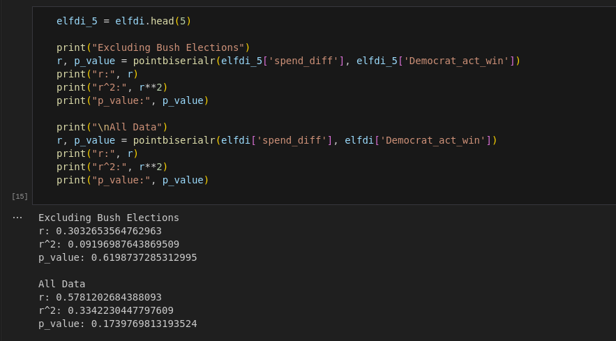
What we see is pretty striking, but not surprising. The p-value suggests no statistical significance. The r and r^2 values similarly suggest weak correlations, but given the small sample size and p-value this could easily be interpreted as no correlation. Excluding the Bush elections gives us a p-value of 0.62, while all elections back to 2000 gives us a p-value of 0.174 (used in the title).
For context, r-values can generally be interpreted as such:
- r = 0.1 to 0.3 might suggest a weak correlation.
- r = 0.3 to 0.7 could be interpreted as a moderate correlation.
- r = 0.7 to 1.0 would indicate a strong correlation.
Negative values are allowed, and they indicate a negative correlation.
Spearman Correlation Coefficient
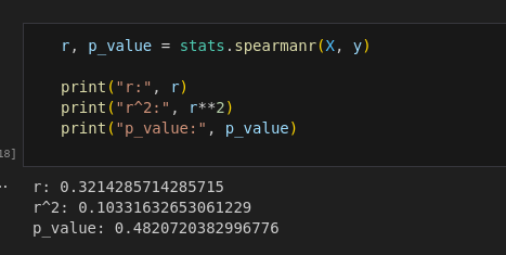
The Spearman test stands out from our biserial test by not requiring normalized data or linearity, which arguably makes it more accurate. It also takes in two continuous variables, allowing us to compare our spending difference against electoral votes. The electoral vote difference isn’t interval scale, however in the spearman test that’s ok.
As expected, we again see essentially no correlation. While our p-value is technically slightly higher (at 0.482), it’s not statistically significant and I would suspect it’s overfitting.
What can we learn from this?
Frankly, we can learn very little, the sample size simply isn’t big enough. While I could go before 2000, I didn’t want to, as I’m afraid elections were too different before then (and the data becomes increasingly sparse).
My finding does agree with other research though, and it makes intuitive sense. Money doesn’t vote, people do, and people often vote for the issues they experience in their everyday lives. In 1980, Jimmy Carter let inflation get to 14%, and in the 1980 November election Ronald Reagan won with 489 electoral votes. In my opinion, no amount of campaign spending was going to get around 14% inflation.
Similarly, in the 2016 election, we saw Russia spend tens of millions on the US election; researchers later determined it had "no measurable changes in attitudes, polarization, or voting behavior".
While I wouldn’t go so far as to say it doesn’t matter, I do think it’s reasonable to conclude that election spending on the US presidential race has very little impact on election results.